


Study of the variation of drilling mud density with temperature, pressure, and circulation rate using artificial neural networks, statistical models, and empirical correlations
- Department of Drilling and Production Engineering, Faculty of Geology and Petroleum Engineering, Ho Chi Minh University of Technology (HCMUT), 268 Ly Thuong Kiet Street, District 10, Ho Chi Minh City, Vietnam
Abstract
Well control is an important aspect of drilling operations because improper well control can result in kicks and blowouts with grave consequences. A successful well control requires a good understanding of the relationships between drilling mud pressure and formation pressure, as well as the variation of bottom hole pressure during drilling operations. As the hydrostatic pressure of the drilling mud column accounts for most of the pressure, a more accurate control of the changes of mud density will contribute to a more accurate bottom hole pressure modeling. Regarding the control of the mud density, a practical problem has existed so far in petroleum drilling: the mud density is determined at the surface condition, and its values vary along the depth of the well because of the changes of temperature and pressure, which consequently leads to an inaccuracy in mud density control in reality.
In order to reduce the inaccuracy in mud density control, this research aims to provide a reliable method to correctly predict the drilling mud’s density under specific conditions. Different artificial neural networks (ANN) were proposed to predict drilling mud density based on the value of mud density at surface conditions, circulation rate, bottomhole pressure, and temperature. This study then used statistical methods to compare the predicted results with results obtained from existing empirical correlations and from other researchers’ works to find out the most optimal artificial neural network which should consist of only one hidden layer. The main contributions of this research in comparison with existing papers are that: 1) Existing methods did not take into account the influence of circulation rate, therefore the real working conditions of the drilling mud were not represented entirely. Our research included the circulating rate in the ANN modeling and in the study of relative importance. The results indicated that the value of mud density at surface conditions had the greatest effect on the prediction results, and the influence of the circulating pump flow rate is small but should not be ignored; 2) Our research used different methods (ANN, Generalized Additive, Nonlinear Function) to predict the mud density in variation with temperature and pressure, which has never been approached in existing literature; 3) The sufficiency in the number of data was studied in this research, which has never been treated in previous studies. The Bootstrap method was used in this regard; 4) We remarked that the overfitting has not been treated properly in the existing literature review in this field, hence we included a thorough analysis of the overfitting in this paper. Finally, the results of this paper can be useful in real life because it can help drillers to accurately predict the mud density under varied conditions of pressure and temperature, and therefore to increase the safety of the drilling operations.
Introduction
Ensuring safety is always the top priority in the oil and gas industry because accidents related to the petroleum sector often lead to loss of time, infrastructure, finance, and manpower. One of the accidents causing severe consequences is the loss of well control during the drilling process, specifically when the pressure in the wellbore is lower than the formation pressure. This scenario can happen if the mud density is not controlled adequately during the drilling operation due to the variation of pressure and temperature inside the wellbore, and consequently the mud density may be too low to maintain bottomhole pressure equal to formation pressure Cormack, 20171. Therefore, being able to accurately calculate the mud density will help to assure a successful drilling operation. In order to achieve this objective, studying the influence of different factors affecting the density of the drilling fluid is extremely necessary.
In literature, there have been various studies relating to the prediction of drilling mud density at different conditions. It is well known that when bottomhole pressure increases, drilling mud density will increase since the drilling fluid volume is compressed, and conversely, when the bottom hole temperature increases, the drilling fluid volume expands leading to a decrease in its density, which is mentioned in Babu, 19962; Hussein and Amin, 20103; An et al., 20154. McMordie et al., 19825 conducted an experimental research about the changes of drilling mud density with temperature (70-400 F) and pressure (0-14000 psi). Similarly, Demirdal & Cunha, 20096 conducted experiments to study the variation of drilling mud density with the same range of pressure (0-14000 psi) but with a different range of temperature (25-175 C). Zamora et al., 20137 also conducted experiments to study the volumetric behavior and the variation of density of base oils, brines, and drilling fluids with the range of temperature (36F–600F) and pressure (0-30000 psi). Some studies provided empirical correlations between mud density and pressure and temperature, such as Kemp, 19898; Peters et al., 19909; Isambourg et al., 199610; Zamora et al., 200011; Hemphill and Isambourg, 200512; and Peng et al., 201613. egarding the application of machine learning in this field, some authors used Artificial Neural Network (Osman et al., 200314; Adesina 201515, Okorie E. Agwu et al., 202016), while some others used different methods such as Fuzzy logic (Ahmadi et al., 201817), Support Vector Machine (Xu et al., 201418; Ahmadi, 201619; Kamari et al., 201720), Radial Basis Function Artificial Neural Network (Rahmati & Tatar, 201921), and Particle Swarm Optimization Artificial Neural Network (Ahmadi et al., 201817; Zhou et al., 201622). It is also worth mentioning the hydraulic model proposed by Charlez et al., 199823 to calculate downhole pressure and then to predict fluid downhole density. In brief, the common point of these studies is to predict drilling mud density at different bottomhole pressures and temperatures.
However, besides temperature and pressure, some other factors also affect the density of drilling fluid, such as the inclination angle of the well which was highlighted in the study of Tian et al., 201324; or the type of drilling fluid which was mentioned in the studies of Demirdal et al., 200725 and Demirdal & Cunha, 20096; and finally the circulation rate which was mentioned in the studies of Kårstad & Aadnøy, 199826 and Harris & Osisanya, 200527. The study of Hemphill, 199628 investigated the effect of inclination angle and of cuttings on drilling fluid properties. Boatman, 196729 studied the influence of shale on drilling fluid density.
In reality, it is challenging to observe the changes in drilling fluid density because of costly specialized measuring equipment which must comply with well design requirements. Ombe et al., 202030 developed a specific measurement to achieve this task. Hoseinpour et al., 202231 combined well logging and geomechanical parameters to determine the mud window, but the authors could not predict the variation of the mud density in function of pressure, temperature, and some other factors.
In brief, the above literature review showed that developing a new method to accurately predict drilling mud density in the well under influence of various factors is necessary, which is the objective of our study. In this study, we resorted to not only machine learning methods but also empirical correlations as well as mathematical, and statistical methods.
Regarding the empirical correlations, Furbish, 199732 provided the following equation of state for liquid density:
(ppg) is predicted drilling mud density, is value of mud density at surface conditions, T and P are final temperature (F) and pressure (psi), T and P are standard temperature (F) and pressure (psi), α (F) is isobaric coefficient and β(F) is isothermal compressibility. These coefficients were taken from the work of Zamora et al. (2000) wherein they used 0.0002546 và 2.823 × 10 for α and β respectively for oil-based mud.
Another empirical correlation given by Hoberock et al., 198233 predicted oil-based mud density and water-based mud through the law of conservation of mass as detailed in the following:
is predicted drilling mud density, (ppg) is value of mud density at surface conditions, (ppg) is initial oil density, (ppg) is oil density in predicted drilling mud, (ppg) is water density in initial drilling mud, (ppg) is water density in predicted drilling mud, (%) is the percentage of oil volume in the drilling fluid, (%) is the percentage of water volume in the drilling fluid.
Kutasov, 198834 presented an empirical correlation to calculate drilling mud density:
(ppg) is the predicted drilling mud density, (ppg) is the drilling mud density at standard conditions. P(psi) and T(F) are standard pressure and temperature. P(psi) and T(F) are the pressure and temperature at the predicted position. Kutasov evaluated α, β, , and with 5 drilling mud examples from McMordie et al., 1982. Besides, Kutasov's correlation can be applied to oil-based mud and water-based mud. In our paper, the values of , and , which were taken from the work of Micah, 201135, were 3.0997 × 10, 2.2139 × 10, and 5.0123 × 10, respectively.
Sorelle et al., 198236 focused on the changes in the volume of the components in drilling fluid caused by temperature and pressure, as being shown in the following formula:
(ppg) is the predicted drilling mud density, (ppg) is the value of mud density at surface conditions, (gal) is the change in oil volume, (gal) is the change in water volume, V(gal) is the total volume.
The literature review allowed us to see some possible contributions that we can bring to the research in this domain. Firstly, the study developed an artificial neural network modeling to predict drilling fluid density, combined with various mathematical, statistical (generalized additive model) and experimental models on the same dataset to provide a comprehensive and multidimensional understanding of the changes in drilling fluid density inside the wellbore. The simulation results were compared with actual data to verify the accuracy of the model.
Secondly, the number of features that our research used for the artificial neural network was greater than in previous studies. As mentioned above, previous papers considered mostly temperature and pressure as input features, while this study presented an artificial neural network modeling with inputs consisting of not only bottomhole temperature and pressure but initial drilling fluid density and circulation rate as well. Consequently, this paper conducted a study about the effect of various influencing factors mentioned above, besides pressure and temperature, on the drilling mud density.
Thirdy, this paper took into account the possible influence of the low number of input data used for ANN modeling. It is difficult to answer the question if a data set is enough for neural networks modeling because the conclusion depends on each particular case. Hence, in this study, we tried to answer this question by using the Bootstrap method to resample the data.
Finally, we remarked that the overfitting analysis was neglected in many previous researches as shown in the above literature review, we therefore included in this paper a thorough solution for the overfitting problem.
The findings of this study have the potential to be applied in real life because they help to improve the accuracy of the mud density’s determination, which in turn will improve the safety of the operations.
Methodology
Mathematical models
Regarding the mathematical models, we initially intended to use a linear function, which is easy to implement, to calculate the drilling mud density based on bottomhole pressure, bottomhole temperature and value of mud density at surface conditions. However, there are some assumptions that we must comply with which can be found in Dahraj & Bhutto, 201437 and Molnar, 202138. The input data was collected from the works of McMordie et al., 19825 and Demirdal & Cunha, 20096, which were summarized in Figure 1. Figure 1 illustrates the variation of drilling mud density in function of temperature and pressure. The blue graph represents the temperature, the orange graph shows the pressure and the green one describes the value of mud density at surface conditions.

The data collected from the works of McMordie et al. (1982) and Demirdal & Cunha (2009) were used in this research for the nonlinear function
Figure 2 to Figure 4 showed that all the histograms of variables are not bell-shaped. Moreover, we also analyzed the distribution of residuals in Figure 5. We observed that the distribution of residuals was not in shape with the red curve, which presented the normal distribution. Instead, the distribution was likely the fat-tailed distribution, which was not normal distribution, so the linear function was not suitable in this case. Consequently, we had to think about another method, which is the nonlinear function, to deal with the problem. This nonlinear function will also be used later to verify the results given by the artificial neural network modeling.

Histogram of bottomhole pressure values (psi)

Histogram of bottomhole temperature values (oF)

Histogram of mud density at surface conditions (ppg)

Histogram of residuals
For the nonlinear function, the quadratic and cubic functions were tested, and we obtained that the correlation coefficient of the cubic function (0.9997) was higher than the one of the quadratic functions (0.9994). In reality, there may be other nonlinear functions with higher correlation coefficients, however, the more complex the function, the higher the risk of overfitting. The cubic function was therefore chosen for this study.
The nonlinear model was constructed by solving the linear least squares problems while using QR factorization which can be referred to the work of Golub & Loan, 199639. The cubic function has the following form:
(ppg) the value of mud density at surface conditions, P and T are pressure (psi) and temperature (F) at the location of interest. The values from A to J were determined and listed in the following:
The nonlinear function presented a high coefficient of determination R = 0.9994. Moreover, the value of mean square error was also accepted, with the MSE = 0.00971 for the nonlinear function (the caluclation of MSE is described in detail in the Appendix section). With input taken from Table 1, the calculated values of drilling mud density (ppg) from empirical correlations and nonlinear function are presented in Table 2.
The input data which was used in this study for empirical correlations and nonlinear function
|
Bottomhole pressure (psi) |
Bottomhole temperature (oF) |
Circulation rate (gal/min) |
Oil volume fraction |
Water volume fraction |
Oil density (ppg) |
Water density (ppg) |
|
8562.279 |
128.55 |
0 |
0.67711 |
0.17524 |
6.6619 |
8.3641 |
|
8671.2 |
128.63 |
0 |
0.67715 |
0.17523 |
6.6603 |
8.3632 |
|
8942.688 |
127.15 |
0 |
0.67684 |
0.17532 |
6.6735 |
8.3717 |
|
8945.111 |
90.74 |
126.8 |
0.67572 |
0.17559 |
6.7226 |
8.4065 |
|
8945.056 |
90.28 |
126.8 |
0.67574 |
0.17558 |
6.7217 |
8.4059 |
|
8946.967 |
90.07 |
126.8 |
0.67574 |
0.17558 |
6.7217 |
8.4059 |
|
8944.121 |
90.02 |
126.8 |
0.67574 |
0.17558 |
6.7216 |
8.4059 |
|
8945.887 |
89.91 |
126.9 |
0.67574 |
0.17558 |
6.7217 |
8.4059 |
Table 2 showed that results obtained from the empirical correlations are close to results obtained from the nonlinear function. Hence, the nonlinear function can be used as an alternative method to predict the drilling fluid density in function of pressure and temperature. However, these methods do not take into account the influence of other factors such as the circulation rate. Hence, in the next section, an artificial neural network modeling will be presented.
Drilling mud density (ppg) obtained from empirical correlations and the nonlinear functions using input data in Table 1
|
Furbish |
Hoberock |
Kutasov |
Sorelle |
Nonlinear function |
|
10.8347 |
11.0440 |
10.8599 |
12.63049 |
10.8949 |
|
10.8378 |
11.0416 |
10.8633 |
12.63005 |
10.8989 |
|
10.8501 |
11.0613 |
10.8771 |
12.63331 |
10.9150 |
|
10.9500 |
11.1354 |
10.9852 |
12.64592 |
11.0635 |
|
10.9513 |
11.1341 |
10.9865 |
12.64577 |
11.0655 |
|
10.9519 |
11.1341 |
10.9871 |
12.64577 |
11.0665 |
|
10.9520 |
11.1340 |
10.9872 |
12.64577 |
11.0666 |
|
10.9523 |
11.1341 |
10.9876 |
12.64577 |
11.0671 |
Machine learning model
Overview of artificial neural network
Artificial Neural Network (ANN) is an artificial intelligence information processing system inspired by the operation of biological neural networks in the human brain. One of the notable features of artificial neural networks is their limited learning ability.
An artificial neural network usually consists of 3 layers and each layer will have a different number of neurons:
-
Input layer: the main function is providing necessary information. A number of neurons in input layer are corresponding to a number of factors and these factors are assumed in the form of vectors
-
Hidden layers contain hidden neurons helping the inputs connect and outputs. A neural network may have one or multiple hidden layers, and in some cases, there is no hidden layer.
-
Output layer includes the neurons which hold output information. A neural network can have many output factors.
Determining the number of hidden layers and the number of neurons is a relatively complex task, there is no rule that finds out the optimal number of hidden layers and hidden neurons. The method of selecting the number of neurons and layers is a trial-and-error approach. The connections between neurons in different layers contain their own individual weights. The number of weights depends on network configuration.
The general relationship between the input data and output data is described below:
x is an input vector, w denotes the connection weight from the ith neuron in the input layer to the jth neuron in the hidden layer, b represents the threshold value or bias of jth hidden neuron, w stands for the connection weight from the jth neuron in the hidden layer to the kth neuron in the output layer, b refers to the bias of the kth output neuron, f and f are the activation functions for the hidden and output neuron, respectively.
The Transfer Function is responsible for transforming the input variable into a different range of values. Some commonly used transfer functions include the logistic sigmoid function, the tangent sigmoid function, and the linear function. Each type of function used has a different purpose for each layer and different types of problems. Nonlinear functions are often used for pattern recognition and discrimination problems and are typically used in the hidden layer. The linear function is used in matching and prediction problems and is usually used in the output layer. This study only covers basic knowledge of machine learning, and readers can refer to additional sources for more information, such as Ghaffari et al., 200640, F. Parrella, 200741, and Mohaghegh, 200042.
Input data for ANN modeling
Input data, which was used to build and calibrate ANN in this study, covered 162 positions of a well at different conditions. The value of drilling mud density at standard conditions is 10.7656 ppg. The data can be viewed in Figure 6.
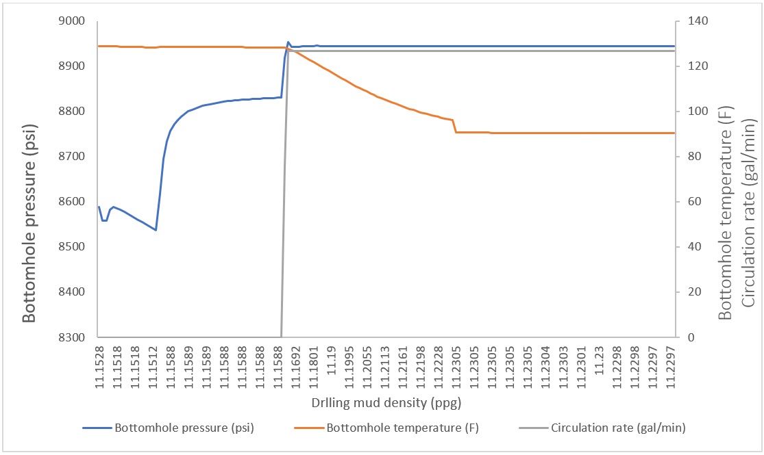
Input data used in this study to build the artificial neural network was provided by Schlumberger in Drillbench software’s tutorial
Artificial neural networks optimization before analysis of overfitting
According to Kårstad & Aadnøy, 199826 and Harris & Osisanya, 200527, the circulation rate also had an effect on drilling mud density. With the desire to contribute a small part to research on predicting drilling mud density, our paper would like to introduce an artificial neural network for predicting drilling fluid density in the function of 4 input factors: surface drilling fluid density, bottom hole pressure, bottom hole temperature, and circulation rate. In the first hidden layer, the transfer function used is the logistic sigmoid function. In the second hidden layer, the transfer function used is the tangent sigmoid function, and in the output layer, the transfer function used is the linear function. This paper used the trial-and-error method to build the networks. Each network structure was run 10 times to avoid random distribution and was selected based on the smallest mean square error in the 10 training runs. In Table 3, with the lowest mean square error MSE , the optimized network consisted of 4 neurons in the input layer, 6 neurons in the first hidden layer, 10 neurons in the second hidden layer, and 1 neuron in the output layer (Figure 7).
However, the solution is not as simple as it seems. We remarked here that the MSE values were anomaly small, which manifested the overfitting problem. Hence, the model can not be used in real life. Therefore, in the following section, we will solve the overfitting problem.
Mean square errors of different networks
|
Layer 1 Layer 2 |
1 neuron |
2 neurons |
3 neurons |
4 neurons |
5 neurons |
6 neurons |
7 neurons |
8 neurons |
9 neurons |
10 neurons |
|
1 neuron |
3.87E-7 |
1.6E-7 |
1.65E-7 |
2.18E-7 |
1.16E-7 |
1.28E-7 |
1.15E-7 |
1.23E-07 |
1.30E-07 |
1.59E-07 |
|
2 neurons |
4.63E-7 |
1.99E-7 |
1.92E-7 |
2.63E-7 |
1.4E-7 |
1.24E-7 |
6.31E-8 |
1.03E-07 |
1.51E-07 |
1.21E-07 |
|
3 neurons |
4.62E-7 |
4.58E-7 |
1.46E-7 |
2.79E-7 |
1.39E-7 |
1.13E-7 |
2.17E-7 |
1.32E-07 |
1.21E-07 |
1.12E-07 |
|
4 neurons |
2.76E-7 |
2.15E-7 |
2.32E-7 |
8.48E-8 |
1.08E-7 |
1.62E-7 |
1.35E-7 |
1.40E-07 |
1.27E-07 |
1.26E-07 |
|
5 neurons |
3.94E-7 |
3.08E-7 |
7.83E-8 |
1.14E-7 |
1.07E-7 |
1.1E-7 |
1.19E-7 |
1.30E-07 |
1.08E-07 |
1.26E-07 |
|
6 neurons |
2.51E-7 |
2.98E-7 |
1.09E-7 |
1.67E-7 |
1.38E-7 |
6.11E-8 |
8.13E-8 |
1.30E-07 |
1.20E-07 |
1.11E-07 |
|
7 neurons |
1.57E-7 |
1.14E-7 |
2.34E-7 |
1.36E-7 |
1.75E-7 |
9.06E-8 |
8.95E-8 |
1.21E-07 |
1.05E-07 |
1.16E-07 |
|
8 neurons |
1.47E-7 |
1.03E-7 |
1.47E-7 |
7.69E-8 |
1.08E-7 |
1.39E-7 |
7.03E-8 |
1.41E-07 |
1.12E-07 |
1.04E-07 |
|
9 neurons |
9.06E-6 |
1.3E-7 |
1.12E-7 |
1.18E-7 |
1E-7 |
1.77E-7 |
6.02E-6 |
1.37E-07 |
1.01E-07 |
1.17E-07 |
|
10 neurons |
1.99E-7 |
8.9E-8 |
1.25E-7 |
1.08E-7 |
1.13E-7 |
5.43E-8 |
1.22E-7 |
1.16E-07 |
1.01E-07 |
1.18E-07 |
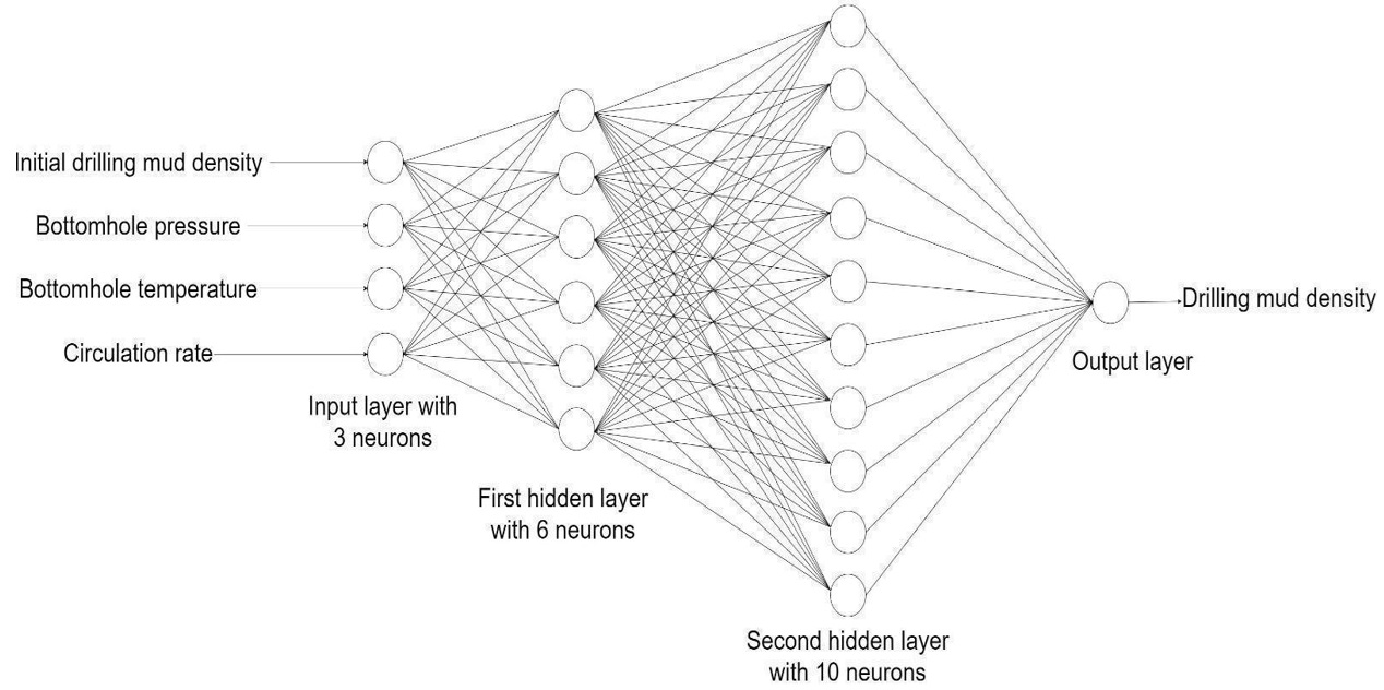
The architecture of the optimized artificial neural network resulted from this study before analysis of overfitting
Solving the overfitting problem and optimizing the artificial neural network.
a. Data pre-processing
The authors knew that the data sets are very important in ANN, that’s why we tried to collect as much data as possible. In this research, we had 327 observations for the non-linear analysis and 162 data for the neural network modeling. Understanding the number of data might be low, hence we referred Horowitzto’s paper in 200843 and conducted the Bootstrap method to resample the data set and obtained a new one with the same statistical characteristics for 400 data points. After that, we divided the data into training set, validation set and test set with proportions of 70%, 15%, 15%, respectively, and used the same ANN models for both original and Bootstrap datasets.
For the targets in neural network training, we used the difference between the density of initial drilling mud and density at bottomhole condition. The input and target data were normalized as shown in the following formulas:
x is a dimensionless value of input data, x is a true value of input data, y is a dimensionless value of target data and y is a true value of target data.
b. Artificial neural networks modeling using Bootstrap data added to original data
Using both original and Bootstrap datasets for the same neural network (3-6-10-1), we observed that the overfitting was decreased (Figure 8) because the MSE values of the test set and validation set were similar. However, in Figure 9, we observed that although the R values obtained from using Bootstrap data was reasonably high (the overfitting problem did not occur), but we also observed that the regression graphs were anormal: many output values fluctuated only around the value of 0.36, which is unusual because in reality the values of target data were more varied. In conclusion, the utilization of Bootstrap method could reduce the overfitting problem, but did not provide satisfactory results. Consequently, in the next section, we will use only original data.
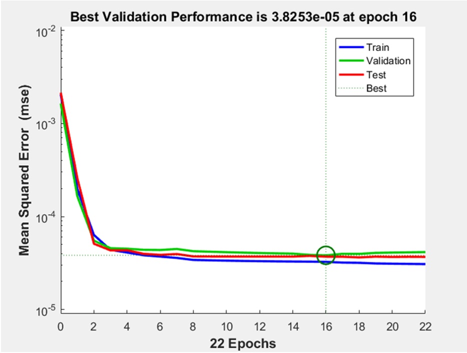
Graph shows the MSE values when using Bootstrap datasets to train the same ANN (3-6-10-1)
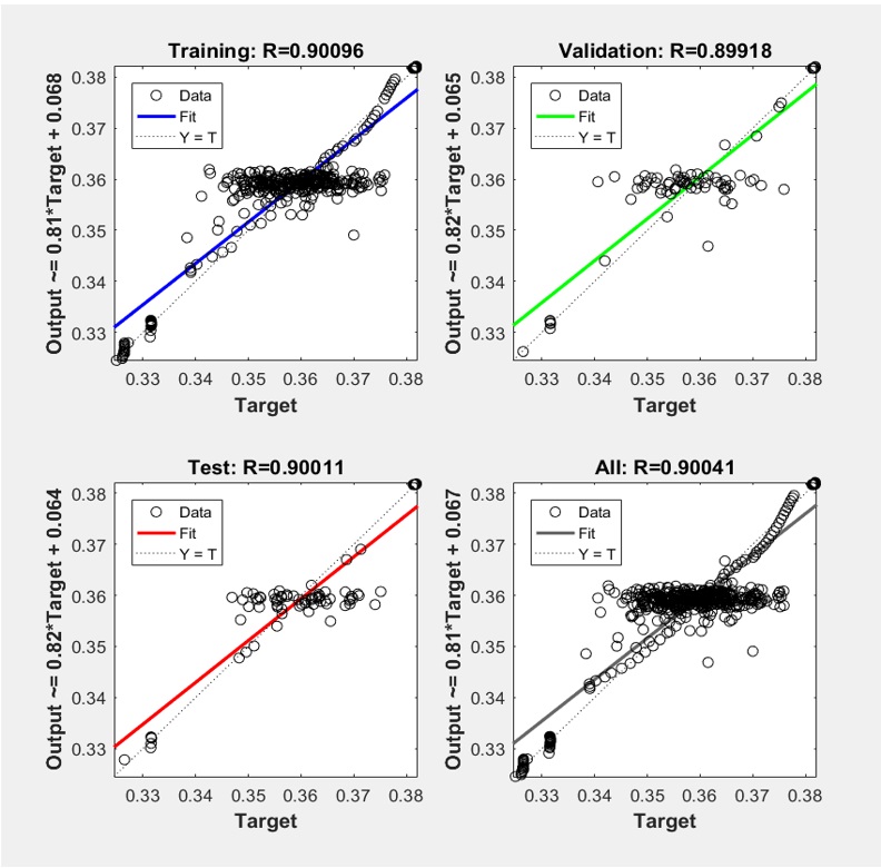
Graph shows the R values when using Bootstrap datasets to train the same artificial neural network
c. Artificial neural networks modeling using only original data with analysis of overfitting
After realizing that the Bootstrap method did not improve the results, the author went back to the normalized original datasets. We then used the same neural network (3-6-10-1), and overfitting was observed in the results: firstly, because the R values were abnormally high (Figure 10); secondly, the MSE of testing set is larger than the one of the training set (Figure 11).
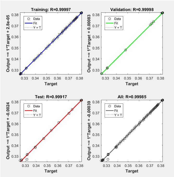
Graph shows the R values when applying the original normalized datasets to the same artificial neural network
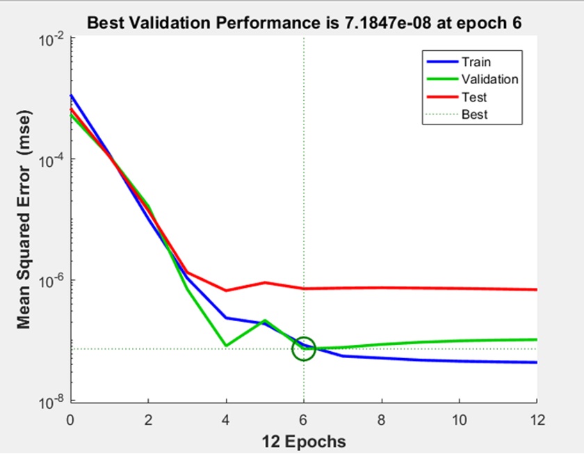
Graph shows the MSE values when applying the original normalized datasets to the same artificial neural network
Therefore, we trained different models which consisted of two hidden layers, and the number of neurons varied from 1 to 10 for each hidden layer. However, the overfitting still existed, so we had to go back to the model with one hidden layer. The results in Figure 12 showed the validation and test curves were very similar, and the MSE of the test set and of the validation set were lower than the one of the train set, which indicated that the overfitting had been excluded. Figure 13 showed that R values and the regression graphs were reasonable without abnormal distribution. In literature, the research of Okorie E. Agwu et al., 202016 possibly had an overfitting problem with very high R value and the predicted values were exactly the same as experimental values. The thorough analysis of overfitting in our research helped to avoid this same problem.
In brief, the results indicated that the optimized network with the best performance without encountering overfitting consisted of one hidden layer with 5 neurons, and the transfer function was tangent sigmoid.
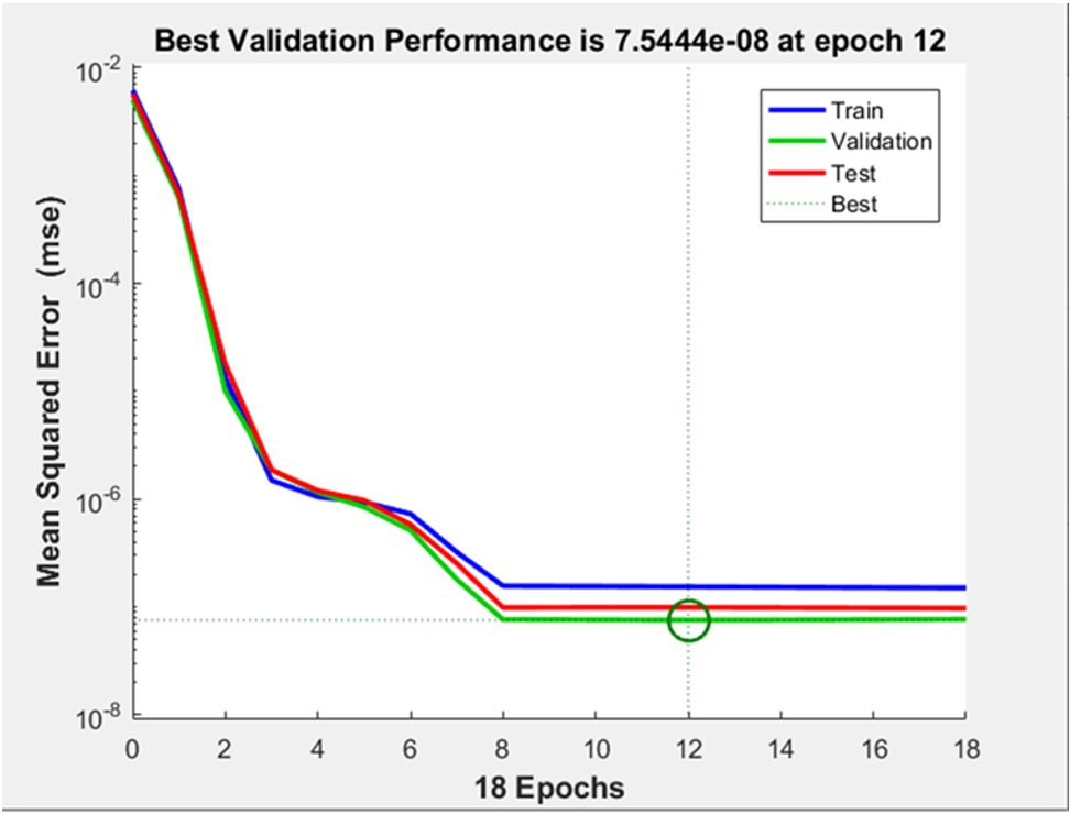
Graph shows the MSE values when applying the original normalized datasets to the artificial neural network with one hidden layer
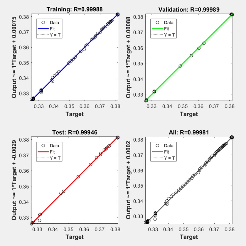
Graph shows the R values when applying the original normalized datasets to the artificial neural network with one hidden layer
The results in previous sections showed that the number of input data is not a problem for ANN modeling as we were afraid at first. There is no simple answer to the question if a data set is enough for neural networks modeling. It really depends on each particular case. The 327 observations for the non-linear analysis and 162 data for the neural network modeling used in this research are therefore enough for a proper analysis. The results showed that we must choose the right neural network model with optimized layers and nodes to have a high accuracy without encountering an overfitting problem. For this case, using one hidden layer is optimized for the ANN modeling. This can be explained by the fact that the more complicated a neural network is, the more data it requires in order to not be overfitted (Muhammad Uzair and Noreen Jamil 202044). Hence, in this study, with our available data, the number of hidden layers must be one, so that no overfitting can occur.
Results and discussion
Since the authors wanted to present various models to predict drilling mud density, a generalized additive model (GAM) was built based on the input data in Figure 6 and evaluated using the same data from Table 1. A generalized additive model is a generalized linear model with a linear predictor involving a sum of smooth functions of covariates (Hastie and Tibshirani 199045). The GAMs can model non-Gaussian outcome variables, in terms of several predictor variables. The requirement of the generalized linear models that the relationships between the outcome and the predictors be linear was relinquished by Vanhove, 201446. Instead, non-linear relationships can also be modeled with the form estimated from the data. This can be accomplished by fitting higher-order polynomial regressions on subsets of the data and adding the pieces together. The more subset regressions are fitted and connected together, the more wiggly the overall curve will be. Fitting too many subset regressions results in overwiggly curves that fit disproportionally much noise in the data (‘oversmoothing’). In order to prevent this, the algorithm can be furnished with a cross-validation procedure or a generalized (algebraic) approximation (Wood, 200647).
Whereas the additive model was estimated by penalized least squares, the GAM will be fitted by penalized likelihood maximization, and in practice this will be achieved by penalized iterative least squares. More specific details can be viewed in the paper of Wood, 200647; Zuur et al., 200948; Vanhove, 201446. Table 4 will show the specific results of drilling mud density obtained from the generalized additive model.
To confirm the effect of circulation rate on the mud density and prove that the network obtained from this study can be applied, the results of drilling mud density obtained from ANN model and generalized additive model were compared with the results from the ANN model of Okorie E. Agwu et al., 202016 in Table 4.
Drilling mud density (ppg) obtained from different artificial neural networks and the generalized additive model using the same input data in Table 1
|
The optimized ANN obtained from this study |
Generalized additive model |
ANN model of Okorie E. Agwu et al. (2020) |
|
11.2358 |
11.1515 |
10.9003 |
|
11.2439 |
11.1603 |
10.9044 |
|
11.2536 |
11.1732 |
10.9199 |
|
11.3584 |
11.2300 |
11.0323 |
|
11.3587 |
11.2302 |
11.0337 |
|
11.3594 |
11.2305 |
11.0345 |
|
11.3585 |
11.2303 |
11.0345 |
|
11.3592 |
11.2305 |
11.0349 |
The determination coefficient between the results obtained from our ANN model and input data is 0.9972, which is rather similar to the determination coefficient (0.9970) obtained from the ANN model of Okorie E. Agwu et al., 202016. However, the mean square error of our network (0.01321) is lower than Okorie E. Agwu’s (0.04754). In addition, as mentioned above, the overfitting problem was included in our analysis, which was not done in Agwu et al., 202016. We concluded that our ANN model provided a high value of coefficient of determination without encountering the overfitting problem. Moreover, the determination coefficient given by the generalized additive model is high (R = 0.99865) while the mean square error is low (3.65 × 10). Hence, our ANN model and generalized additive model can be used in real life applications.
Eventually, Table 6 showed that almost all of the methods were reliable. Only the calculated results given by Sorelle et al., 198236 gave a significant deviation compared to the input data, hence using the model of Sorelle is not highly recommended. Although the determination coefficient of our ANN model is lower than the one given by the generalized additive model, the ANN method can still be accepted because of its small mean square error (Table 5), and because it can include more influence factors in the input data than the other methods.
Figure 14 shows the predicted results obtained from different methods that were used in this study. The measured data in Figure 6 were the same data as the input data used in ANN modeling. Figure 14 allowed us to draw the same conclusions as mentioned in the previous paragraph.
The results of drilling mud density (ppg) obtained from the optimized ANN, generalized additive model, and empirical correlations for the same input data from Table 1
|
Nonlinear function |
Generalized additive model |
Furbish |
Hoberock |
Kutasov |
Sorelle |
The optimized ANN obtained from this study |
|
10.8949 |
11.1515 |
10.8347 |
11.0440 |
10.8599 |
12.63049 |
11.2358 |
|
10.8989 |
11.1603 |
10.8378 |
11.0416 |
10.8633 |
12.63005 |
11.2439 |
|
10.9150 |
11.1732 |
10.8501 |
11.0613 |
10.8771 |
12.63331 |
11.2536 |
|
11.0635 |
11.2300 |
10.9500 |
11.1354 |
10.9852 |
12.64592 |
11.3584 |
|
11.0655 |
11.2302 |
10.9513 |
11.1341 |
10.9865 |
12.64577 |
11.3587 |
|
11.0665 |
11.2305 |
10.9519 |
11.1341 |
10.9871 |
12.64577 |
11.3594 |
|
11.0666 |
11.2303 |
10.9520 |
11.1340 |
10.9872 |
12.64577 |
11.3585 |
|
11.0671 |
11.2305 |
10.9523 |
11.1341 |
10.9876 |
12.64577 |
11.3592 |
Comparison of correlation coefficients and errors given by different methods
|
Statistical parameters |
MSE |
RMSE |
|
Methods | ||
|
The optimized ANN obtained from this study |
0.01321 |
0.1149 |
|
ANN model of Okorie E. Agwu et al. (2020) |
0.04754 |
0.2180 |
|
Furbish |
0.08631 |
0.2938 |
|
Hoberock |
0.01023 |
0.1011 |
|
Nonlinear function |
0.04083 |
0.2021 |
|
Kutasov |
0.06892 |
0.2625 |
|
Sorell |
2.06639 |
1.4375 |
|
Generalized additive model |
3.65E-06 |
0.0019 |

Graph shows results of drilling mud density (ppg) obtained from empirical correlations, nonlinear function, generalized additive model, and machine learning models
Study of relative importance of different input parameters
Analyzing the impact of the three factors (pressure, temperature, and surface density) using the nonlinear mathematical model
To analyze the impact of the three factors, which are pressure, temperature, and surface density, input data in Figure 1 was used for the evaluation with help of the Equation (5). The effect of these three factors are illustrated in Figure 15. We observed that if the value of mud density at surface conditions is reduced to 60%, the drilling mud density at the wellbore conditions will decrease to approximately 55%. Another remark is that if the bottomhole temperature is reduced to 60%, the drilling mud density will increase by approximately 1.05 times. Besides, if the bottomhole pressure is reduced to 60%, the drilling fluid density will be 0.95 compared to the initial value.
These above observations are similar to the ones discussed in the works of Agwu et al. 202016 and Osman et al., 200314. Both of these two papers concluded that surface density had the biggest impact, followed by bottomhole temperature and bottomhole pressure.
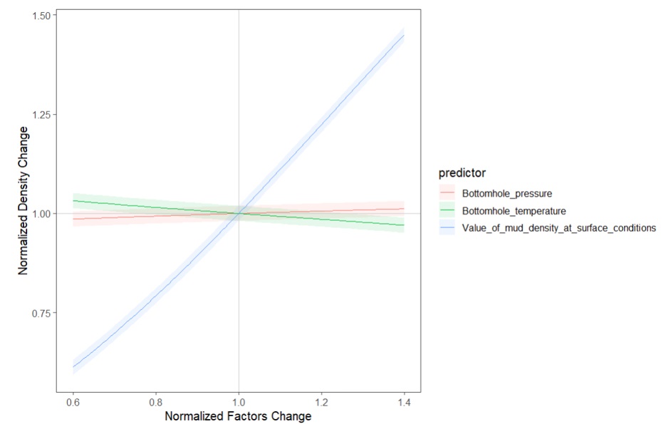
Relative importance of bottomhole pressure, bottomhole temperature, and the value of mud density at surface conditions to the drilling mud density
Analyzing the impact of the four factors (pressure, temperature, surface density, and circulation rate) using generalized additive model
Since the value of mud density at surface conditions is constant during the operation, it may not be wise to include it in the study. Therefore, instead of considering the impact of surface drilling fluid density on the bottomhole drilling mud density, we evaluated another factor which was the circulation rate. Harris and Osisanys, 200527 mentioned that the circulation rate was proportional to the drilling fluid density at the bottomhole condition because higher flow rates would cause the bottomhole pressure to increase and the bottomhole temperature to decrease. Besides that, no study about the influence of circulation rate has ever been realized so far.
Our generalized additive model was used to study the level of variables’ importance with help of the data presented in Figure 6. Figure 16 showed that the effect of the circulation rate on the drilling mud density was quite low. Combined with the results shown in the previous section, it can be concluded that the level of influence of different factors on the drilling fluid density is in the following order: value of mud density at surface conditions, bottomhole pressure, bottomhole temperature, and circulation rate.
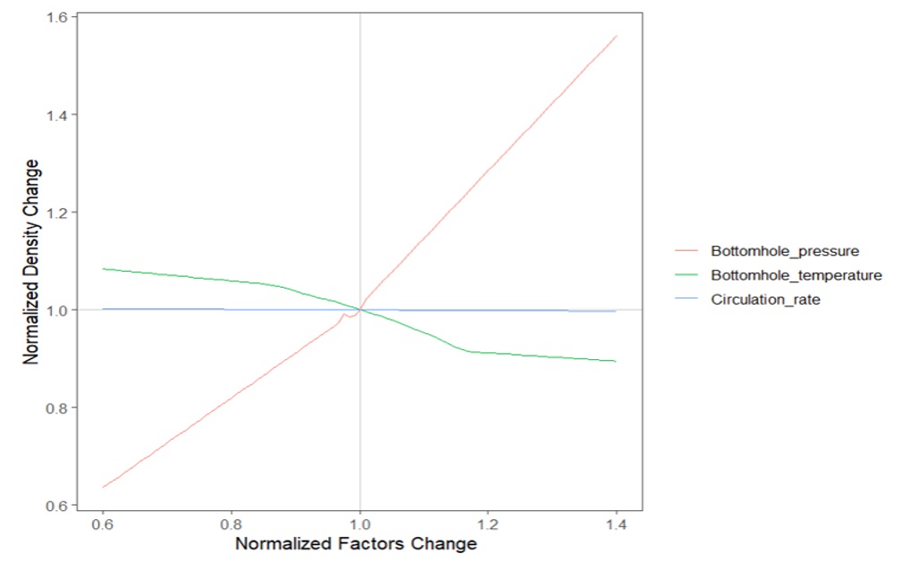
Relative importance of bottomhole pressure, bottomhole temperature, and circulation rate to the drilling mud density
Conclusions
This paper presented various methods (artificial neural network, generalized additive model, nonlinear function, empirical correlations) to predict drilling mud density in function of temperature, pressure, surface value of the drilling fluid, and circulation rate. The results lead to the following conclusions:
-
The Generalized Additive model and Artificial Neural Network have higher coefficient of determination R2 and lower MSE than the other methods. However, it is recommended to use our optimized ANN method because we demonstrated that it did not have a problem of overfitting, while the Generalized Additive model presented a very low MSE, which should be used with caution.
-
The optimized ANN model consisted of only one hidden layer. In addition, the answer to the question if a data set is enough for neural networks modeling is not simple because it depends on each particular case. In this study, the Bootstrap method was used to resample the data and the conclusion was that the number of input data was enough to avoid the overfitting problem. Moreover, it is worthy to note that since there was often a lack of overfitting analysis in previous studies in literature review regarding this specific case, we solved this problem by conducting a thorough analysis of overfitting in this paper.
-
The nonlinear model is more appropriate than the linear model in this case based on the analysis of the histograms of different variables.
-
The empirical correlations presented higher deviation between predicted results and measured data, especially the correlation given by Sorelle et al. (1982).
-
The level of impact on drilling mud density is in the following order: value of mud density at surface conditions, bottomhole pressure, bottom hole temperature, and circulation rate.
ABBREVIATIONS
ANN: Artificial neural network
: Percentage of oil volume in the drilling fluid
: Percentage of water volume in the drilling fluid
GAM: Generalized additive model
MSE: Mean Squared Error
(psi): Standard pressure
(psi): Pressure at the predicted position
RMSE: Root Mean Squared Error
(F): Standard temperature
(F): Temperature at the predicted position
V (gal): Total volume
(gal): Difference in oil volume
(gal): Difference in water volume
: A true value of input data
: A maximum value of input data
: A minimum value of input data
: A dimensionless value of input data
: A true value of target data
: A dimensionless value of target data
(ppg): Value of mud density at surface conditions
(ppg): Predicted drilling mud density
(ppg): Initial oil density
(ppg): Oil density in predicted drilling mud
(ppg): Initial water density
(ppg): Water density in predicted drilling mud
CONFLICT OF INTEREST
The authors declare that there are no conflicts of interest in the publication of this article.
AUTHORS’ CONTRIBUTION
Pham Son Tung directed and supervised the development and completion of the research, as well as reviewed and revised the article.
Pham Thanh Nhacollected data, built the models, and drafted the manuscript.
APPENDIX
Mean Squared Error (MSE) is a formula for estimating the squared value of an error. The smaller the value of MSE, the more accurate the prediction is.
Root Mean Square Error (RMSE) is used to evaluate how well a model fits the data. When the value of RMSE is near 0, the model will be more accurate.
T-value is a measure that indicates the degree of influence of input factors on the results. The absolute value of the t-value indicates the greater the degree of influence. A negative t-value indicates an inverse relationship between the input factor and the result, and vice versa.
The correlation coefficient is a statistical parameter that measures the degree of fit between predicted and actual data of drilling fluid density.
N is the total number of observations, I is the index of I observation; X* is the value of drilling mud density which is predicted from empirical correlations or machine learning models.
Pr (>|t|) is the p-value corresponding to the t-value. If the p-value is less than the statistical significance level α (usually 0.05), the factors associated with it will be statistically significant in the results, otherwise, it will be a random factor.