


Build-up an analysis model to evaluate wind potential for selecting suitable turbine configurations and proposing research to optimize wind farm design
- Ho Chi Minh City University of Technology, Vietnam
- VietNam National University HCM City, Vietnam
Abstract
Before a wind farm is constructed, the assessment of wind potential in the proposed turbine installation area must be carried out as a prerequisite. To achieve the highest efficiency, the key concepts and a deep understanding of wind energy evaluation must be mastered by the design engineers. The article of study applies Weibull distribution theory and aerodynamics fundamental to build an analytical model for evaluating standards and estimating annual electricity output based on raw input data collected over a year. The calculation results for the wind characteristics, including shape and scale factor and power density at the surveyed area corresponding to an 80m height, are determined in detail by simulation software. The analysis results also indicate that the wind potential here is classified as very high (class 6), and a minimum II-A type turbine configuration must be selected to withstand these wind conditions.
Since the initial investment cost of a wind farm will be determined by the simulation results, the study aims to combine the calculation methods used in this research with the application of digital twin solutions and machine learning for wind farms to create an accurately digital replica of a physical system. In this way, real-time system operations will be monitored and continuously updated into the simulation model to understand and predict its behavior. From there, optimal design and operation adjustments will be made to enhance the overall system's efficiency and minimize errors and risks for investors.
Introduction
Recently, within the national strategy on Climate Change, the Vietnamese government has announced the goal of reducing emissions by 43.5% by 2030, with practical proposal and effective international support. Emission targets have been set for each sector for the years 2030 and 2050, alongside several qualitative proposals to achieve these goals. Among these proposals are policies to support the development of wind power projects in Vietnam1.
To construct a wind power plant, the first requirement is to have a basic knowledge of wind energy. Specifically, whether a wind power project is grid-connected or standalone, the core activity to assess the feasibility of the project is the Wind Resource Assessment (WRA) process2. The output data from WRA will be used and serve as the input for financial analysis and the overall feasibility assessment of entire project 3.
Currently, wind farms are increasingly being developed, offering significant opportunities to enhance autonomous operation and optimize system productivity. In light of these, the research has developed an annual energy production (AEP) analysis model to select suitable turbine configurations 4.
This analytical model plays a vital role in providing estimated electricity generation results with high reliability and accuracy of 100% when the characteristic parameters of the input wind dataset are identified. Additionally, the model also assists in predicting energy sources at different altitudes when planning designs to aid in feasibility assessments. The research results will provide a more detailed and intuitive perspective on providing useful scientific information that serves as a valuable reference for future wind power projects.
INPUT DATA AND METHODOLOGY
Data source
The input data consist of wind speed measurements taken every 10 minutes continuously over one year at the Con Dao telecommunications station as in Figure 1 at altitudes of 30m, 50m, and 60m above ground level respectively.
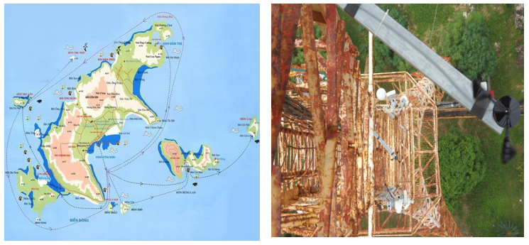
The Con Dao Island map and picture of installation of anemometer at altitudes of60m, 50m & 30m
Based on these gathered wind speed data series, which to be presented in the form of Table 1 and chart as shown in Figure 2 to analyze and evaluate the characteristic of the avarage hourly wind speed at diffferent elevation.
Hourly average wind speed at different elevation
|
Hour |
Wind speed (hourly average), m/s | ||
|
60m (Channel 1) |
50m (Channel 2) |
30m (Channel 3) | |
|
0 |
6.32 |
5.68 |
4.18 |
|
1 |
6.14 |
5.51 |
4.07 |
|
2 |
6.10 |
5.47 |
4.05 |
|
3 |
6.25 |
5.60 |
4.14 |
|
4 |
6.32 |
5.66 |
4.19 |
|
5 |
6.52 |
5.85 |
4.34 |
|
6 |
6.60 |
5.92 |
4.37 |
|
7 |
6.77 |
6.07 |
4.49 |
|
8 |
7.03 |
6.30 |
4.67 |
|
9 |
7.23 |
6.49 |
4.82 |
|
10 |
7.45 |
6.68 |
4.93 |
|
11 |
7.61 |
6.83 |
5.05 |
|
12 |
7.72 |
6.92 |
5.11 |
|
13 |
7.90 |
7.08 |
5.21 |
|
14 |
8.03 |
7.20 |
5.33 |
|
15 |
8.13 |
7.29 |
5.40 |
|
16 |
8.07 |
7.23 |
5.35 |
|
17 |
7.95 |
7.13 |
5.25 |
|
18 |
7.84 |
7.04 |
5.20 |
|
19 |
7.62 |
6.83 |
5.06 |
|
20 |
7.29 |
6.54 |
4.85 |
|
21 |
7.02 |
6.30 |
4.66 |
|
22 |
6.73 |
6.03 |
4.45 |
|
23 |
6.55 |
5.87 |
4.34 |
|
Average |
7.13 |
6.40 |
4.73 |
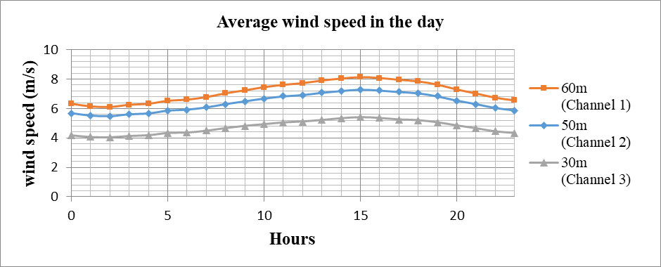
Hourly average wind speed in year (from 0h to 23h) at observed heights.
Methodology
In this study, an experimental method is proposed by collecting and processing data along with a mathematical method of probabilistic statistical analysis. According to the Weibull distribution is used to determine the importantly characteristic parameters of wind. Thermodynamic properties of moist air also is applied to build a simulation model by using MATLAB software to provide predictive results and potential assessment.
The classification of turbines according to the IEC-1400-1 standard is determined by average wind speed and turbulence intensity. The IEC-1400-1 standard defines four standard classes: I, II, III, IV, and an additional class S. For class S, all wind field parameters must be specified by the manufacturer. The average wind speeds for classes I through IV correspond to 10 m/s, 8.5 m/s, 7.5 m/s, and 6 m/s, respectively. In addition to these standard classes, turbulence intensity is categorized into high, medium, and low (classes A, B, and C).
THE ANALYSIS MODEL FOR EVALUATION AND ESTIMATING ANNUAL ELECTRICITY OUTPUT
The kinetic energy (E) of the wind in moving can be determined as the formular5
(3-1)
where m is the mass of air passing through a circular plane perpendicular to the wind direction and ν is the mean wind speed over a suitable time period that can be seen in Figure 3 .
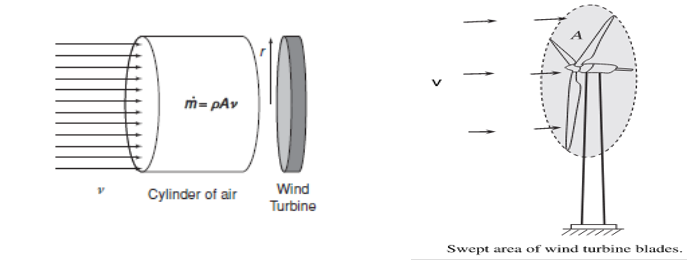
Kinetic energy and swept area of wind turbine
The wind power can be obtained by differentiating the kinetic energy in wind with respect to time:
However, only a small portion of wind power can be converted into electrical power. When wind passes through a wind turbine and drives blades to rotate, the corresponding wind mass flowrate is:
Where ρ is density of a moist air (kg/m) and A is the swept area of blades (m)
From above formula of (3-2) and (3-3), simplifying this we get a power (P) can be expressed as 5 :
The effective power through a wind turbine for electricity generation is significantly less than the energy in the air stream. According to Betz’s law, theoretically, only a maximum of 59,3% of the energy in the air stream can be captured because the wind speed behind a turbine cannot be fully absorbed and reduced to zero.
Statistical modeling of wind speed data
The statistical modeling method is applied the Weibull probability distribution as a crucial form to describe the statistical appearance of extreme values in meteorology, hydrology and weather forecasting. The Weibull distribution provides a reasonable mathematical description for wind speed graphs. This distributon is used to analyze probability, predict operational time, and estimate the electricity generation.
The Weibull probability density function :
Where:
k: Shape factor
A: Scale factor
Below frequency distribution graphs are created by grouping wind speeds. The shape parameter k and the scale parameter A allow the Weibull function to be fitted to the measured frequency distributions. Each region will have different k and A values, as illustrated in Figure 4, Figure 5 .
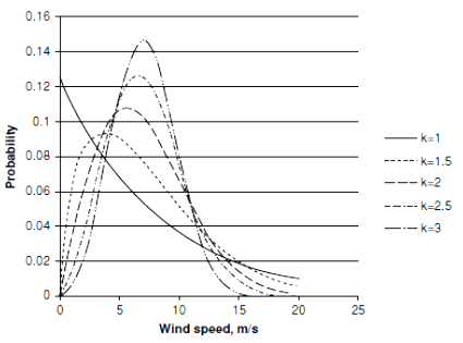
Weibull probability density function according to k-values
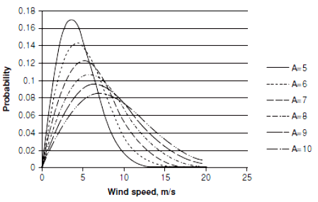
Weibull probability density function according to A-values
Power density of wind speed
To understand the inpact of the statistical distribution of wind speed on power generation, we need to calculate this power density of wind speed.
Power density (PD) is defined as follow:
However, this PD value must be applied integral function to achieve result more accurate:
Where: v is wind speed (m/s), pd(v) is Weibull probability density function
Conventionally, wind intensity in the surveyed area is classified based on power density to evaluate the wind energy potential of that specific area. To assess this potential, wind speeds are categorized into 7 levels according to Table 2 . Based on the calculated power density using formula 3-6, we can determine whether that area has wind potential or not.
Wind classification at reference heights 10m & 50m
|
Wind Class |
Category |
10m |
50m | ||
|
Power density2 |
Average velocity |
Power density2 |
Average velocity | ||
|
1 |
Poor |
0-100 |
0-4.4 |
0-200 |
0.0-5.6 |
|
2 |
Marginal |
100-150 |
4.4-5.1 |
200-300 |
5.6-6.4 |
|
3 |
Fair |
150-200 |
5.1-5.6 |
300-400 |
6.4-7.0 |
|
4 |
Good |
200-250 |
5.6-6.0 |
400-500 |
7.0-7.5 |
|
5 |
Excellent |
250-300 |
6.0-6.4 |
500-600 |
7.5-8.0 |
|
6 |
Outstanding |
300-400 |
6.4-7.0 |
600-800 |
8.0-8.8 |
|
7 |
Superb |
400-1000 |
7.0-9.4 |
800-2000 |
8.8-11.9 |
Air density correction according to ambient temperature
Typically, wind energy is surveyed at ambient temperature. Air density (ρ) is also a factor that affects power density (PD). The relationship between PD and ρ is linear. Air density depends on pressure, temperature and relative humidity, both pressure and temperature decrease with altitude. The formula for calculating air density is obeyed the perfect gas equation of state as follows 7 :
Where:
-
p: atmospheric pressure, (atm)
-
V: total mixture volume (i.e dry air & water vapor), (m3)
-
n: number of moles of air (mol)
-
R: universal gas constant, 8,314 J/(mol.K)
-
T: absolute temperature, (K)
With ρ = n/V, molecular weight per volume unit.
Hence, the term M (gam) represents the molecular weight of air. Air density is defined in below formula:
Otherwise, the pressure depends on altitude. The pressure value may be calculated from 5, 8 :
Where:
M: the molecular weight of air, (M = 28.97 g/mol)
Z: altitude, m
This correction is necessary for wind energy assessment at different altitudes.
Wind speed distribution by Altitude
Wind speed is typically measured at a specific altitude above the sea level as indicated in Figure 6. However, to enhance the efficiency of wind energy utilization, it is sometimes necessary to consider wind speeds at various heights. The equation for velocity as a function of altitude is expressed by the formula:
Where:
v,v is the wind speed at height h, h, respectively
γ is the wind shear exponent, which varies depending on the terrain and atmospheric conditions.
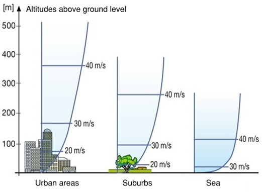
Wind speed distribution by height
In case of considering to extrapolate wind speed, γ-coefficient may be determined as follows:
Additionally, in cases of lacking observational input data, we can refer to the Table 3 to find γ coefficient for each specific condition.
Terrain’s roughness classification & wind shear coefficient
|
Terrain Description |
Roughness Class |
Roughness length, m |
Wind Shear Coefficient , γ |
|
Offshore sea |
0 |
0.0001 – 0.003 |
0.08 |
|
Open terrain, smooth surface (concrete roads, short grass) |
0.5 |
0.0024 |
0.11 |
|
Agricultural land without obstacles, sparse buildings, or a few hills |
1 |
0.03 |
0.15 |
|
Agricultural land with few houses and tree fences 8m tall spaced 1250m apart |
1.5 |
0.055 |
0.17 |
|
Agricultural land with few houses and tree fences 8m tall spaced 500m apart |
2 |
0.1 |
0.19 |
|
Agricultural land with few houses and tree fences 8m tall spaced 250m apart |
2.5 |
0.2 |
0.21 |
|
Villages, small towns, agricultural land with many tall trees, rough terrain |
3 |
0.4 |
0.25 |
|
Large cities with many high-rise buildings |
3.5 |
0.8 |
0.31 |
|
Large cities with many skyscrapers |
4 |
1.6 |
0.39 |
Correlation between characteristic parameters of the Weibull
In addition to the two characteristic parameters k and A factor of Weibull distribution. We may establish other relationship of wind speed as follow:
Where: Γ(x) is gamma function, if x is an integer then Γ(x) = x!
To simplify this, we may apply the approximate formula as below:
ANALYTICAL RESULT OF WIND POTENTIAL ASSESSMENT AND TURBINE CONFIGURATION SELECTION
Frequency of wind speed levels
Wind speed data for determining frequency of occurrence
Based on the collected wind data series, the wind data will be summarized in a chart that shows the frequency of occurrence corresponding to speeds ranging from less than 1m/s to 25m/s at a typical height of 60m (see Figure 7 ).
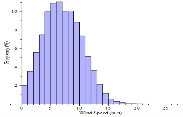
The statistical frequency of actual wind speed at the height of 60m
The analysis and observations of the wind speed frequency
-
The frequency of wind speeds from 6m/s and above accounts for 60,5%.
-
The maximum observed wind speed is 31,59m/s (recorded from the max channel of anemometer).
Statistical characteristics of the data series for
Data for determining statistical characteristics
Based on the 10 minute average wind speed data series, the statistical characteristics of the observed wind data will be calculated by using the Weibull distribution function. Applying the formulas to calculate k, A and PD. The results in Figure 8 at a height of 60m are as follows:
-
Air density at 60m:
-
Shape factor: k = 2,23
-
Scale factor: A = 8,03
-
Average wind speed: 7,12 m/s
-
Mode = 6.17 m/s
-
Standard deviation: σ = 3.36 m/s
-
Power density: PD = 363,15 W/m2
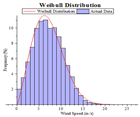
Characteristics of actual wind speed data at 60m follow Weibull Distribution
Analysis and Observation
With an average power density of approximately 363,15 W/m at 60m, according to the Table 2 then the wind potential of this area is classified into class 3 which is very suitable for energy exploitation. When a wind turbine is installed at a height of 80m, its potential will be even better.
Wind Speed Data Conversion
Since the statistical data series of wind speed is not available at 80m, it is necessary to extrapolate and convert from the surveyed data series at other heights.
Based on the collected data series, applying formula 3-13 to find out γ value which allows for the conversion of wind speed. To verify the accuracy of γ-coefficient, the statistical data series at a height of 60m is used to convert wind speeds at 30m and 50m respectively. These converted data are then compared and evaluated against actual data at these heights to conclude the reasonableness of the chosen γ value. Using this method, the converted and statistical data values are listed in Table 4 and illustrated in Figure 9.
Average hourly windspeeds throughout the Year at observed heights of the statistical data seriesand calculated converted data
|
Hour |
Actual data series |
Converted data according to heights |
Wind Shear γ | |||||
|---|---|---|---|---|---|---|---|---|
|
60m |
50m |
30m |
80m |
60m |
50m |
30m | ||
|
0 |
6.32 |
5.68 |
4.18 |
7.52 |
6.32 |
5.67 |
4.18 |
0.601 |
|
1 |
6.14 |
5.51 |
4.07 |
7.30 |
6.14 |
5.51 |
4.07 |
0.599 |
|
2 |
6.10 |
5.47 |
4.05 |
7.25 |
6.10 |
5.47 |
4.04 |
0.597 |
|
3 |
6.25 |
5.60 |
4.14 |
7.44 |
6.25 |
5.60 |
4.13 |
0.603 |
|
4 |
6.52 |
5.66 |
4.19 |
7.52 |
6.32 |
5.66 |
4.17 |
0.603 |
|
5 |
6.52 |
5.85 |
4.34 |
7.75 |
6.52 |
5.85 |
4.32 |
0.598 |
|
6 |
6.60 |
5.92 |
4.37 |
7.85 |
6.60 |
5.92 |
4.36 |
0.600 |
|
7 |
6.77 |
6.07 |
4.49 |
8.05 |
6.77 |
6.07 |
4.48 |
0.601 |
|
8 |
7.03 |
6.30 |
4.67 |
8.35 |
7.03 |
6.30 |
4.65 |
0.599 |
|
9 |
7.23 |
6.49 |
4.82 |
8.59 |
7.23 |
6.49 |
4.79 |
0.597 |
|
10 |
7.45 |
6.68 |
4.93 |
8.87 |
7.45 |
6.68 |
4.92 |
0.603 |
|
11 |
7.61 |
6.83 |
5.05 |
9.05 |
7.61 |
6.83 |
5.04 |
0.599 |
|
12 |
7.72 |
6.92 |
5.11 |
9.19 |
7.72 |
6.92 |
5.10 |
0.600 |
|
13 |
7.90 |
7.08 |
5.21 |
9.40 |
7.90 |
7.08 |
5.21 |
0.604 |
|
14 |
8.03 |
7.20 |
5.33 |
9.56 |
8.03 |
7.20 |
5.30 |
0.602 |
|
15 |
8.13 |
7.29 |
5.40 |
9.66 |
8.13 |
7.29 |
5.38 |
0.598 |
|
16 |
8.07 |
7.23 |
5.35 |
9.60 |
8.07 |
7.23 |
5.33 |
0.603 |
|
17 |
7.95 |
7.13 |
5.25 |
9.47 |
7.95 |
7.12 |
5.25 |
0.601 |
|
18 |
7.84 |
7.04 |
5.20 |
9.32 |
7.84 |
7.04 |
5.20 |
0.599 |
|
19 |
7.62 |
6.83 |
5.06 |
9.05 |
7.62 |
6.83 |
5.04 |
0.601 |
|
20 |
7.29 |
6.54 |
4.85 |
8.66 |
7.29 |
6.54 |
4.83 |
0.597 |
|
21 |
7.02 |
6.30 |
4.66 |
8.35 |
7.02 |
6.30 |
4.65 |
0.600 |
|
22 |
6.73 |
6.03 |
4.45 |
8.00 |
6.73 |
6.03 |
4.45 |
0.599 |
|
23 |
6.55 |
5.87 |
4.34 |
7.78 |
6.55 |
5.87 |
4.33 |
0.599 |
|
Mean |
7.13 |
6.40 |
4.73 |
8.48 |
7.13 |
6.40 |
4.72 |
0.60 |
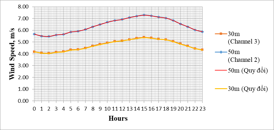
Average hourly wind speeds throughout the year at observed heights and converted
As the result inTable 4 and Figure 9 , the error between the calculated converted data and actual collected data is negligible and entirely acceptable. All curve lines representing these data are almost coincident.
Conclusion: Using the formula to calculate γ-coefficient for converting wind speed at a height of 80m is accepted.
Variation of Average Hourly Wind Speed Throughout the Year at 80m Height
Average Hourly Wind Speeds Throughout the Year at 80m Height, Extrapolated from the Statistical Data Series
|
Average Hourly Wind Speeds, m/s |
Average Hourly Wind Speeds, m/s | |||
|
Hours |
80m (Extrapolated) |
Hours |
80m (Extrapolated) | |
|
0 |
7.52 |
13 |
9.40 | |
|
1 |
7.30 |
14 |
9.56 | |
|
2 |
7.25 |
15 |
9.66 | |
|
3 |
7.44 |
16 |
9.60 | |
|
4 |
7.52 |
17 |
9.47 | |
|
5 |
7.75 |
18 |
9.32 | |
|
6 |
7.85 |
19 |
9.05 | |
|
7 |
8.05 |
20 |
8.66 | |
|
8 |
8.35 |
21 |
8.35 | |
|
9 |
8.59 |
22 |
8.00 | |
|
10 |
8.87 |
23 |
7.78 | |
|
11 |
9.05 |
Average |
8.48 | |
|
12 |
9.19 | |||
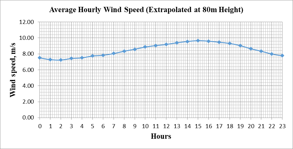
Average Hourly Wind Speeds Throughout the Year at 80m Height, Extrapolated from the Statistical Data Series
Characteristic Parameters of the Data Series for Calculation
Based on the 10-minute average wind speed data series collected at heights of 30m, 50m, and 60m, the extrapolation of wind data to a height of 80m was carried out as indicated in Table 5 and Figure 10). The wind data characteristics were derived using the Weibull distribution function, similar to the method used for the 60m height. The results are illustrated in Figure 11 and Figure 12.
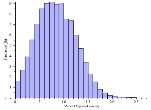
The statistical frequency of converted wind speed at the height of 80m
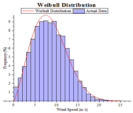
Characteristics of wind speed data at 80m follow Weibull Distribution
Where:
-
Air density at 80m: ρ = 1,167 kg/m3
-
Shape factor: k = 2,23
-
Scale factor: A = 9,55
-
Average wind speed: 8,46 m/s
-
Mode = 7.32 m/s
-
Standard deviation: σ = 4.0 m/s
-
Power density: PD = 608,29 W/m2
Observation:
With an average power density of approximately 608.29 W/m² at a height of 80 meters, the wind potential of this area is very high and classified into class 6. Comparing the results at heights of 60m and 80m, it is evident that the higher the altitude, the greater the energy potential. Therefore, installing wind turbine at a height of 80 meters is very reasonable.
Selection of Turbine Based on Power Generation Capacity and Annual Electricity Production Estimation
Selection of Power Generation Capacity
The selection of the wind turbine’s power generation capacity should align with the load demand requirement. Refer to the hourly load demand Table 6.
Where:
-
Max load demand, Pmax = 4,580.48 kW
-
Min load demand, Pmin = 2,479.26 kW
-
Ave. load demand, Pave = 3,617.22 kW
From the Table 6 of given load data, to ensure a stable power supply for the island and minimizing dependence on the previous diesel system to reduce greenhouse gases, a turbine capacity should be selected greater than the peak load. Here, the total system capacity of 5MW is chose as shown in Figure 13.
Hourly Load DemandSummary at Con Dao Island
|
Hours |
Load Demand, KW |
Hours |
Load Demand, KW | |
|
1 |
4,580.48 |
13 |
4,059.10 | |
|
2 |
2,958.77 |
14 |
3,701.82 | |
|
3 |
2,479.26 |
15 |
4,421.96 | |
|
4 |
2,501.59 |
16 |
3,514.80 | |
|
5 |
2,764.47 |
17 |
3,779.97 | |
|
6 |
3,322.21 |
18 |
3,668.32 | |
|
7 |
3,391.99 |
19 |
4,212.62 | |
|
8 |
3,782.76 |
20 |
3,403.07 | |
|
9 |
4,070.26 |
21 |
3,679.40 | |
|
10 |
3,715.77 |
22 |
3,763.14 | |
|
11 |
4,156.79 |
23 |
3,768.72 | |
|
12 |
4,112.13 |
24 |
3,003.92 |
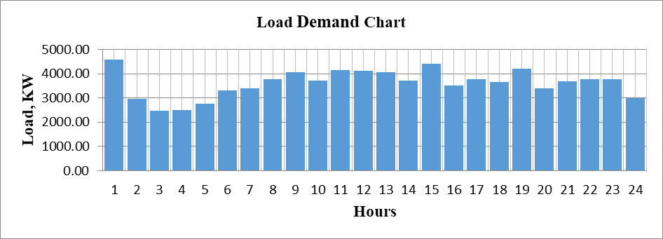
Hourly Load Demand Summary at Con Dao Island
Basis for selecting wind turbine capacity:
-
The selected turbine capacity must meet the load demand and ensure uniform distribution.
-
The power penetration level from the wind power system must achieve at least 50%.
-
It should align with the financial capacity of the investor.
-
Under the same conditions, the harmonization between technical aspects and investment costs must be taken into account.
-
A backup plan must be considered in case one of the devices needs maintenance or replacement.
Conclusion:
Above these criteria, the most suitable configuration is to choose 2 turbines with a capacity of 2.5 MW each, totalling 5 MW.
Estimation of Annual Electricity Production
Wind speed frequency simulation result
To accurately determine the number of hours per year that the wind speed reaches between v and v, the following equation can be used
(4-1)
Where:
8760: Total number of hours in a year.
f(v): The probability density function of wind speed
Based on the collected statistical data and the extrapolated wind speed results at a height of 80m, the parameters of Weibull distribution can be found:
-
k = 2,23
-
A = 9,55
Applying the above formula with the determined values of k, A. The wind speed frequency tabulated in Table 7 and shown in Figure 14.
Wind speed frequency according to Weibull distribution
|
Wind Speed Frequency According to Weibull Distribution | |||
|
v = 0 |
m/s |
0.00 |
h/year |
|
v = 1 |
m/s |
126.64 |
h/year |
|
v = 2 |
m/s |
289.98 |
h/year |
|
v = 3 |
m/s |
456.48 |
h/year |
|
v = 4 |
m/s |
607.53 |
h/year |
|
v = 5 |
m/s |
728.70 |
h/year |
|
v = 6 |
m/s |
809.99 |
h/year |
|
v = 7 |
m/s |
846.50 |
h/year |
|
v = 8 |
m/s |
838.70 |
h/year |
|
v = 9 |
m/s |
791.84 |
h/year |
|
v = 10 |
m/s |
714.73 |
h/year |
|
v = 11 |
m/s |
618.14 |
h/year |
|
v = 12 |
m/s |
512.99 |
h/year |
|
v = 13 |
m/s |
408.92 |
h/year |
|
v = 14 |
m/s |
313.31 |
h/year |
|
v = 15 |
m/s |
230.85 |
h/year |
|
v = 16 |
m/s |
163.61 |
h/year |
|
v = 17 |
m/s |
111.55 |
h/year |
|
v = 18 |
m/s |
73.18 |
h/year |
|
v = 19 |
m/s |
46.19 |
h/year |
|
v = 20 |
m/s |
28.05 |
h/year |
|
v = 21 |
m/s |
16.39 |
h/year |
|
v = 22 |
m/s |
9.21 |
h/year |
|
v = 23 |
m/s |
4.98 |
h/year |
|
v = 24 |
m/s |
2.59 |
h/year |
|
v = 25 |
m/s |
1.29 |
h/year |
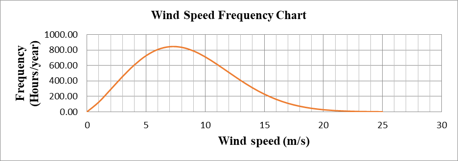
Occurrence wind speed frequency chart at 80m
Power Generation Characteristics of the Wind Turbine
For the selected wind turbine with a power capacity of 2.5MW, refer to the typical power output (P) of Enercon manufacturer 9 according as wind speed (v). The power curve of a turbine 2.5 MW is as Table 8.
The power curve and operating data of the wind turbine 2.5 MW catalogue
|
The Characteristic Curve of Wind Turbine 2.5 MW | |||
|
v = 0 |
m/s |
0.0 |
kW |
|
v = 1 |
m/s |
0.0 |
kW |
|
v = 2 |
m/s |
3.0 |
kW |
|
v = 3 |
m/s |
48.0 |
kW |
|
v = 4 |
m/s |
153.0 |
kW |
|
v = 5 |
m/s |
335.0 |
kW |
|
v = 6 |
m/s |
620.0 |
kW |
|
v = 7 |
m/s |
1023.0 |
kW |
|
v = 8 |
m/s |
1530.0 |
kW |
|
v = 9 |
m/s |
2015.0 |
kW |
|
v = 10 |
m/s |
2350.0 |
kW |
|
v = 11 |
m/s |
2480.0 |
kW |
|
v = 12 |
m/s |
2500.0 |
kW |
|
v = 13 |
m/s |
2500.0 |
kW |
|
v = 14 |
m/s |
2500.0 |
kW |
|
v = 15 |
m/s |
2500.0 |
kW |
|
v = 16 |
m/s |
2500.0 |
kW |
|
v = 17 |
m/s |
2500.0 |
kW |
|
v = 18 |
m/s |
2500.0 |
kW |
|
v = 19 |
m/s |
2500.0 |
kW |
|
v = 20 |
m/s |
2500.0 |
kW |
|
v = 21 |
m/s |
2500.0 |
kW |
|
v = 22 |
m/s |
2500.0 |
kW |
|
v = 23 |
m/s |
2500.0 |
kW |
|
v = 24 |
m/s |
2500.0 |
kW |
|
v = 25 |
m/s |
2500.0 |
kW |
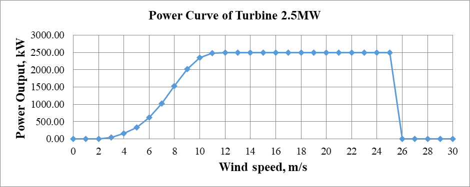
Power output characteristic curve of a typical turbine 2.5MW
In the given Table 8, the cut-in wind speed at which the wind turbine start operating is 2m/s, the power output of the wind turbine increases rapidly as the wind speed increases respectively. The turbine reaches its rated power and maintain as it at 12m/s. When the wind speed exceeds 25m/s, the wind turbine automatically activates its protection system for cut-out, ensuring the safety of the equipment (see Figure 15).
Estimation of annual electricity production
The annual electricity production of a wind turbine is the product of its power output (P) and the operating time in one year. From the statistical Table 9, the annual electricity production can be estimated as Table 9.
Annual electricity production from wind turbine 2.5 MW
|
v = 0 |
m/s |
- |
kWh/year |
|
v = 1 |
m/s |
- |
kWh/year |
|
v = 2 |
m/s |
869.95 |
kWh/year |
|
v = 3 |
m/s |
21,911.16 |
kWh/year |
|
v = 4 |
m/s |
92,951.72 |
kWh/year |
|
v = 5 |
m/s |
244,115.47 |
kWh/year |
|
v = 6 |
m/s |
502,194.42 |
kWh/year |
|
v = 7 |
m/s |
865,974.01 |
kWh/year |
|
v = 8 |
m/s |
1,283,211.33 |
kWh/year |
|
v = 9 |
m/s |
1,595,547.53 |
kWh/year |
|
v = 10 |
m/s |
1,679,626.08 |
kWh/year |
|
v = 11 |
m/s |
1,532,990.03 |
kWh/year |
|
v = 12 |
m/s |
1,282,466.94 |
kWh/year |
|
v = 13 |
m/s |
1,022,298.84 |
kWh/year |
|
v = 14 |
m/s |
783,283.68 |
kWh/year |
|
v = 15 |
m/s |
577,120.43 |
kWh/year |
|
v = 16 |
m/s |
409,020.14 |
kWh/year |
|
v = 17 |
m/s |
278,885.35 |
kWh/year |
|
v = 18 |
m/s |
182,954.05 |
kWh/year |
|
v = 19 |
m/s |
115,477.28 |
kWh/year |
|
v = 20 |
m/s |
70,124.48 |
kWh/year |
|
v = 21 |
m/s |
40,966.07 |
kWh/year |
|
v = 22 |
m/s |
23,020.26 |
kWh/year |
|
v = 23 |
m/s |
12,441.33 |
kWh/year |
|
v = 24 |
m/s |
6,465.85 |
kWh/year |
|
v = 25 |
m/s |
3,230.81 |
kWh/year |
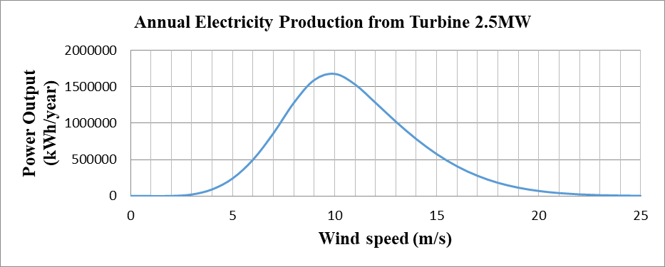
Annual electricity production chart of a 2.5MW Wind Turbine
-
As seen in Figure 16, the annual electricity production from a 2.5 MW turbine produces approximately 12.644 million kWh/yr. Therefore, the total production from the system will be around 25.29 million kWh/yr.
-
Maximum operating hours (Tmax) is 12.64 x10⁶/2500 = 5057.41 hr/yr.
Calculation of Turbulence Intensity and
To select the appropriate wind turbine capacity for installation at a specific area, the turbulence intensity of wind speed must be considered carefully (see Figure 17). It reflects the level of random fluctuation in wind speed. It depends on the terrain surface and obstacles encountered by the wind on its flow path.
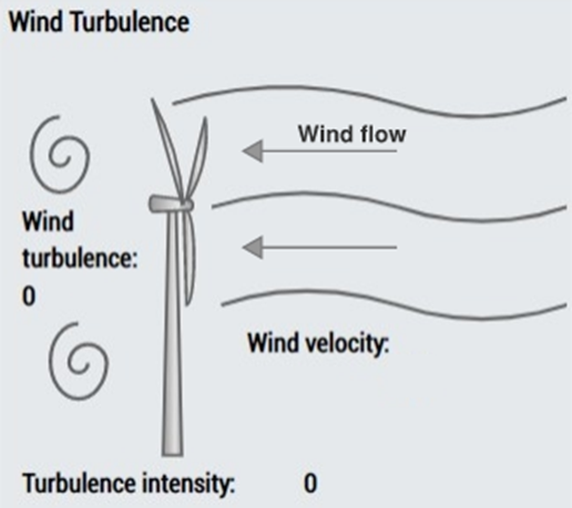
Model of wind flow and wind turbine
The basic formula for determining turbulence intensity10:
Where:
I : Turbulence intensity, (%)
σ: Standard deviation of wind speed (m/s)
v : the individual wind speed measurement, (m/s)
: average wind speed (m/s)
This turbulence directly affects to lifespan of the turbine. Therefore, the IEC 61400-1 standard defines wind turbine classification as Table 10.
Wind Turbine Classification following IEC standard
|
Basic parameters for the standard WTG classes I-IV | |||||||
|
WTG Class |
I |
II |
III |
IV | |||
|
Parameters |
Vref |
(m/s) |
50 |
42.5 |
37.5 |
30 |
Values specified by Designer |
|
Vave |
(m/s) |
10 |
8.5 |
7.5 |
6 | ||
|
A |
Iref |
0.16 | |||||
|
B |
Iref |
0.14 | |||||
|
C |
Iref |
0.12 | |||||
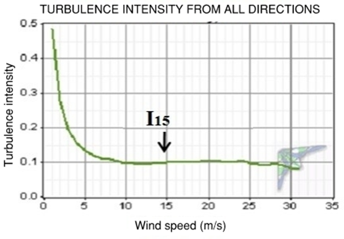
Where, V = V/0.2 and I is calculated at referred wind speed of 15m/s as indicated in Figure 18 according to the installation height.
From standard deviation channel of wind speed, the apparent turbulence intensity (ATI) is calculated by using formula 4-2:
Result of the Apparent Turbulence Intensity
|
Wind speed (m/s) |
Ave. Turbulence Intensity, (TI ave) |
Standard Deviation (ST) |
Apparent Turbulence Intensity, (ATI) |
|
v = 1 |
0.7555 |
1.3320 |
2.4604 |
|
v = 2 |
0.7296 |
0.4342 |
1.2854 |
|
v = 3 |
0.5010 |
0.2497 |
0.8206 |
|
v = 4 |
0.3652 |
0.1681 |
0.5803 |
|
v = 5 |
0.2893 |
0.1264 |
0.4511 |
|
v = 6 |
0.2374 |
0.1020 |
0.3680 |
|
v = 7 |
0.2023 |
0.0819 |
0.3072 |
|
v = 8 |
0.1817 |
0.0687 |
0.2696 |
|
v = 9 |
0.1613 |
0.0574 |
0.2348 |
|
v = 10 |
0.1474 |
0.0504 |
0.2120 |
|
v = 11 |
0.1474 |
0.0504 |
0.2120 |
|
v = 12 |
0.1357 |
0.0412 |
0.1883 |
|
v = 13 |
0.1321 |
0.0391 |
0.1822 |
|
v = 14 |
0.1288 |
0.0377 |
0.1770 |
|
v = 15 |
0.1269 |
0.0375 |
0.1748 |
|
v = 16 |
0.1206 |
0.0371 |
0.1682 |
|
v = 17 |
0.1133 |
0.0380 |
0.1619 |
|
v = 18 |
0.1098 |
0.0376 |
0.1579 |
|
v = 19 |
0.1015 |
0.0389 |
0.1514 |
|
v = 20 |
0.0942 |
0.0356 |
0.1397 |
|
v = 21 |
0.0883 |
0.0412 |
0.1411 |
|
v = 22 |
0.0922 |
0.0395 |
0.1428 |
|
v = 23 |
0.0859 |
0.0318 |
0.1266 |
|
v = 24 |
0.0839 |
0.0318 |
0.1246 |
|
v = 25 |
0.0594 |
0.0251 |
0.0915 |
|
v = 26 |
0.0607 |
0.0110 |
0.0749 |
Where:
Column TI is the value of average turbulence intensity according to wind speed v.
Column ST is a standard deviation of TI and to be calculated as the following formula 11:
Where: n is the number of measurements
is an average of the individual measurement and the formula can also be expressed as 11:
Column ATI is the apparent turbulence intensity. According to the Table 1012, value of ATI is calculated as follows:
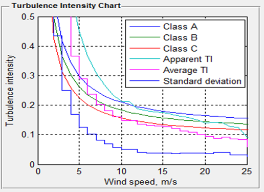
Calculated result of apparent turbulence intensity and 03 curves according to IEC.
Based on the calculated results in Table 11 and can be seen in the Figure 19 , the ATI wind speed of 15m/s is 17.48%. According to the IEC standard, the reference turbulence intensity I is defined as:
Applying above formula 4-6, the I is calculated approximately 15.56%.
The average wind speed at a height of 80m is 8.46m/s. According to the IEC, the reference wind speed is calculated as:
V = V/0.2 = 42.3m/s.
By comparing V and I with Table 10, the selected turbine class for installation is Class II-A.
Observation:
The right selection of turbine class is crucial, if choosing a lower class could affect turbine’s performace due to unexpected wind gusts. Conversely, selecting a higher class turbine would increase the initial investment costs.
In order to validate the calculated both k and A value from section Statistical characteristics of the data series for energy calculation, the results in Figure 20 were cross-checked by using the WindPro software (see Figure 21) for comparision and verification with the same input data.
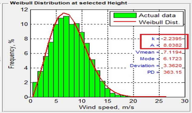
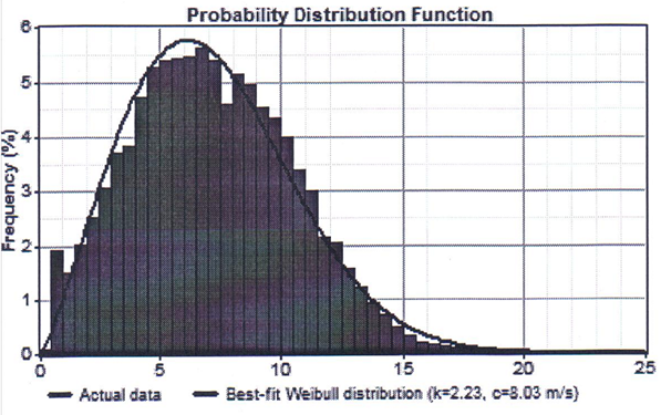
Calculated results of characteristic parameters from WindPro 2.5
-
Conclusion
In terms of methodology, it can be observed that the results of the characteristic parameters are the same, affirming the reliability of the simulation software programmed. This is considered a critical step in assessment the feasibility of an entire wind power project.
CONCLUSION AND DISCUSSION
To avoid inaccurate forecasts and increased experimental costs that waste resources, each wind farm project, both existing and planned for the future, must be performed in detailed analysis. By creating computational models as illustrated in Figure 22, we establish a basis for assessing the wind energy potential of a given area and data, estimating the maximum annual electricity production a turbine can generate with highly reliable and accurate analysis results, and ultimately evaluating turbulence intensity conditions to select the appropriate turbine type for the intended installation site.
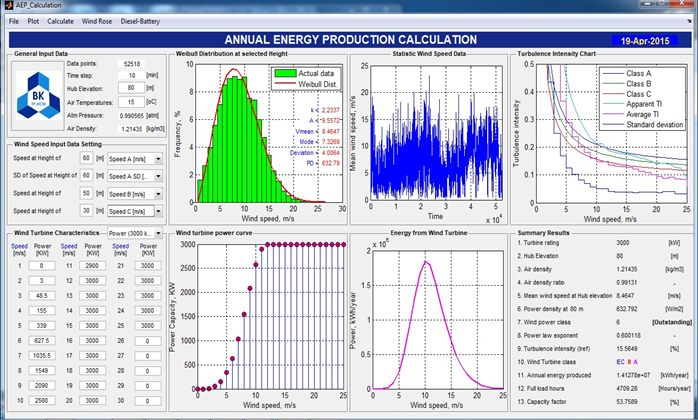
The Analytical Modelof Annual Energy Potential Calculation.
Furthermore, to optimize the design and operation of the system in the future, the research proposes the development of digital twin (see Figure 23) and machine learning applications for wind farms13. This involves establishing Physics-based models to simulate operating conditions under various scenarios (what-if simulations) due to the continuous changes in input variables. Such analyses will enable appropriate adjustments to enhance the overall system efficiency. The benefits of digital twin somution include:
-
Optimizing the placement of wind turbines to maximize wind energy capture.
-
Increasing the electricity output of the wind farm.
-
Reducing operational and maintenance costs.
-
Extending the lifespan of the equipment.
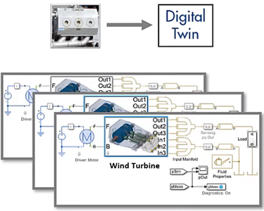
Digital twin modelcan predict failures and optimal design adjustment
Finally, the development of a hybrid model that combines Physics-based modeling and machine learning is proposed. This model will learn from actual operational data, improving and enabling an evaluation of the performance of system components and providing more accurate and optimal adjustment signals 14,15.
Competing Interests
We hereby confirm that there are no conflicts of interest regarding the entire content of this paper.
Authors' Contributions
Truong Trong Hieu: Collected input data, processed and performed data analysis, developed algorithms, and built analytical software with graphical visualization, wrote and revised the manuscript.
Nguyen The Bao: Advise mathematical formulas and contributed to manuscript revision.